Tips & Tricks, Tutorials, Hacking, Troubleshooting,

Showing posts with label Excel. Show all posts

Excel is such a powerful spreadsheet program that I doubt anyone can possibly know everything that it can do. There are so many aspects to the program, it’s amazing that it can all be encapsulated in such a simple interface. I was recently using Excel for some work at home and found myself using the IF function to write a few formulas.
Being able to write a simple IF statement in Excel is essential, especially if you deal with a lot of numbers all the time. It’s one of those things that’s not too complicated like macros, but not necessarily intuitive like summing up a column of numbers.
In this article, I’ll walk you through a short primer on writing a IF statement in an Excel worksheet. To get started, you should understand the basis of all IF statements:
IF condition THEN true ELSE false
That’s pretty much it. The condition is usually a comparison of something. That something is normally numbers or text. We’ll start off with some basic number comparisons, then text, then include operators like AND/OR, etc. So here’s our first example:
simple if formula
We have a very simple example here. Two columns with two numbers, 25 and 35. If Column C, we want to check if Column A is greater than 10, we will output the text Yes, otherwise the text No. A few things to note:
1. You don’t have to put a set of parenthesis around the actual comparison, but it’s very good practice, especially when the comparison becomes more complicated.
2. To output text for the true or false value, you have to use double quotes. If you don’t, it will think you are trying to refer to a named range in Excel.
Now let’s see some more stuff you can do. In the comparison section, you can also do math too. For example, you can do this if you like:
if statement
Here we are saying that if the value of A2 times 10 is greater than 10, then output Yes, otherwise output No. Pretty straight-forward eh? Now let’s say we wanted to output numbers instead of text. Here’s one example:
excel if statement
In this example, if the value in A2 is greater than 10, it will output the value times 2, otherwise it will multiply the value by 5. Pretty useless, but you get the point. You can also use the value of other cells too in the formula.
if formula
Here we are saying that if the value of A2 is greater than 10, then multiple B2 by 10, otherwise multiple B2 by 5 and output that value into cell C2. Now let’s make it more complicated. What if we wanted to output Yes if both A2 and B2 are greater than 10?
excel if
Here’s something new! If we want A2 > 10 AND B2 > 10, then we have to use the AND function inside the IF function. Sounds tricky, but not too bad. The AND function basically takes multiple comparison arguments (A2 > 10) and does an AND on them. They all have to be true in order for “Yes” to be displayed. You can add three or four or more comparison arguments if you like. If you want to do an OR, simply replace the AND above with the word OR.
What about if you want to return a value other than text or a calculated number. What if you want to return the value of a cell on a different sheet? Well, you can do something like this:
return value sheet
For the true value, I am going to return the value of cell A1 on Sheet 2. That’s pretty easy! So you can easily reference values from other sheets if you like. In the same light, you can also use a value from another sheet in the logical comparison too, i.e. Sheet2!A1 > 10. Let’s look at more stuff you can do! Let’s say you wanted to do an IF statement based on the type of value stored in a cell (number, text, or blank). You can do something like this:
isblank excel
You can use ISTEXT and ISNUMBER for the other two types of data. These functions can be really convenient when writing IF formulas. Note that you can basically use most functions in Excel inside of a IF statement, so feel free to run loose. For example, you can use functions like SUM, MAX, MIN, etc.
So far we’ve only been working with one value in the logical comparison, but let’s say we want to work with a group of cells. For example, if all the numbers in a range of cells is greater than 10, output True, otherwise False.
range cells excel
It’s as simple as using the colon like shown above, A2:A4. In this case, each value from A2 to A4 will be tested to see if it’s greater than 10. If all of them are, then the true value will be displayed. What about nested IF statements?
nested if
Here, I am saying that if A2 is greater than 10, output a value, but if not, then perform another IF comparison. IF B2 is greater than 10, then output a different value. You can nest IF statements 64 levels deep, which means you can do some pretty complicated stuff. You’ll probably never need to go that far, but sometimes it’s useful a few levels deep.
This is only a basic introduction to the IF statement, but hopefully it’ll get you started. Are you trying to write an IF statement to do something in Excel and can’t figure it out? Post a comment here with the problem and I’ll try to help you write the proper IF formula. Enjoy!
Although Excel’s long list of functions is one of the most enticing features of Microsoft’s spreadsheet application, there a few underutilized gems that enhance these functions. One often-overlooked tool is the What-If Analysis.

Excel’s What-If Analysis tool is broken down into three main components. The part discussed here is the powerful Goal Seek feature that lets you work backwards from a function and determine the inputs necessary to get the desired output from a formula in a cell. Read on to learn how to use Excel’s What-If Analysis Goal Seek tool.

Excel’s Goal Seek Tool Example

Suppose that you want to take out a mortgage loan to buy a house and you are concerned about how the interest rate on the loan will affect the yearly payments. The amount of the mortgage is $100,000 and you will pay back the loan over the course of 30 years.

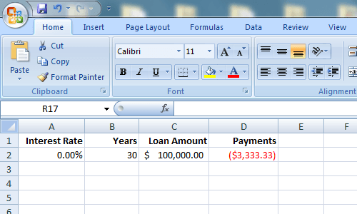
Using Excel’s PMT function, you can easily figure out what the yearly payments would be if the interest rate were 0%. The spreadsheet would likely look something like this:

A Simple Mortgage Payment Calculation in Excel

The cell at A2 represents the yearly interest rate, the cell at B2 is the length of the loan in years, and the cell at C2 is the amount of the mortgage loan. The formula in D2 is:

=PMT(A2,B2,C2)

and represents the yearly payments of a 30-year, $100,000 mortgage at 0% interest. Notice that the figure in D2 is negative since Excel assumes that the payments are a negative cash flow from your financial position.

Unfortunately, no mortgage lender is going to lend you $100,000 at 0% interest. Suppose you do some figuring and find out that you can afford to pay back $6,000 per year in mortgage payments. You are now wondering what is the highest interest rate you can take on for the loan to make sure you don’t end up paying more than $6,000 per year.

Many people in this situation would simply start typing numbers in cell A2 until the figure in D2 reached approximately $6,000. However, you can make Excel do the work for you by using the What-If Analysis Goal Seek tool. Essentially, you will make Excel work backwards from the result in D4 until it arrives at an interest rate that satisfies your maximum payout of $6,000.

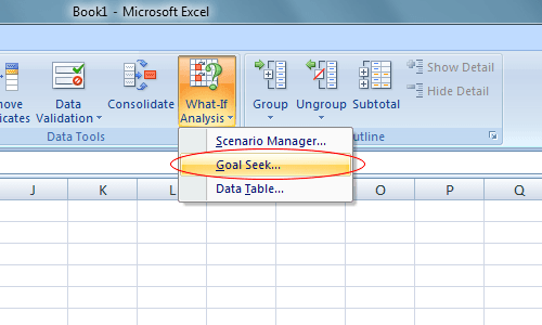
Begin by clicking on the Data tab on the Ribbon and locating the What-If Analysis button in the Data Tools section. Click on the What-If Analysis button and choose Goal Seek from the menu.

Excel What-If Analysis Goal Seek Tool

Excel opens up a small window and asks you to input only three variables. The Set Cell variable must be a cell that contains a formula. In our example here, it is D2. The To Value variable is the amount you want the cell at D2 to be at the end of the analysis.

For us, it is -6,000. Remember that Excel sees payments as a negative cash flow. The By Changing Cell variable is the interest rate you want Excel to find for you so that the $100,000 mortgage will cost you only $6,000 per year. So, use cell A2.

Excel Goal Seek Variables

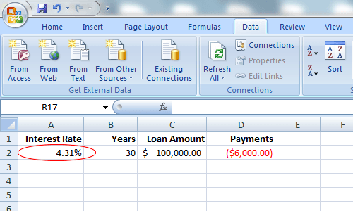
Click the OK button and you may notice that Excel flashes a bunch of numbers in the respective cells until the iterations finally converge on a final number. In our case, the cell at A2 should now read about 4.31%.

Results from an Excel What-If Goal Seek Analysis

This analysis tells us that in order not to spend more than $6,000 per year on a 30-year, $100,000 mortgage, you need to secure the loan at no more than 4.31%. If you want to continue doing what-if analyses, you can try different combinations of numbers and variables to explore the options you have when trying to secure a good interest rate on a mortgage.

Excel’s What-If Analysis Goal Seek tool is a powerful complement to the various functions and formulas found in the typical spreadsheet. By working backwards from the results of a formula in a cell, you can explore the different variables in your calculations more clearly.

If you’ve used Excel for any length of time, you know that this spreadsheet application is as adept at manipulating strings of text as it is at manipulating numbers. When it comes to functions, however, Excel users tend to be more familiar with the ones that compute new numbers than those that change text.

If you have two strings of text and want to combine them into one cell, you can use the Concatenate function to do just that. Behaving just like any other function in Excel, the Concatenate function lets you join strings of text rather than compute numbers.

Using Excel’s Concatenate Function

Let’s say you have an Excel worksheet that contains people’s addresses. When you originally entered the addresses, you put the number of the address in one cell and the street on another. Now, you want to combine the number and street into one string.

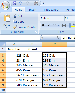
Sample Address Excel Spreadsheet

In the sample spreadsheet pictured above, suppose you want the combined street numbers and street names to appear in the column next to each pair. This is exactly the situation where using the Concatenate function is useful.

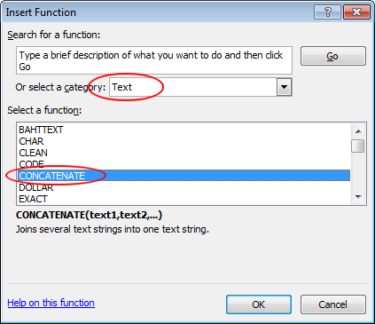
Begin by clicking on the C3 cell and then clicking on the Function button next to the formula bar. On the Or Select a Category drop menu, select Text and locate and click on the function titled Concatenate. Then, click the OK button

Select Text and Then Concatenate

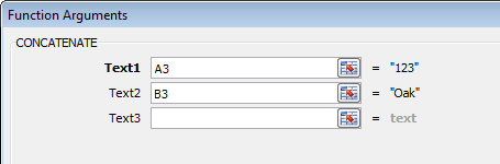
Excel will then open up the familiar Function Arguments window where you can type in or select a cell or range of cells to include in the current formula. In the Text1 box, type in A3 and in the Text2 box, type in B3. Then, click the OK button.

Excel Function Arguments Window

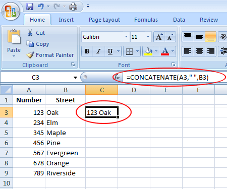
You’ll notice that Excel has created a new entry in cell C3 that is a concatenation of cells A3 and B3. However, there is a problem because the 3 and the O in Oak are right next to each other. To conform to the standard, you need a space between the numbers and the letters of the address. Rather than put the space in manually, you can force Excel to put a space between concatenated text.

Make sure C3 is the active cell and go to the function bar. Edit the formula so that is looks like this:

=CONCATENATE(A3,” “,B3)

Notice that there is a space between the open and closed quotation marks. Press the Enter key and the address in cell C3 will now have a space between the number 3 and the O in Oak.

Put a Space Between Concatenated Text

Now, you can simply drag the square in the box around C3 down to cell C9 to concatenate the rest of the addresses in the spreadsheet.

Drag the Excel Function Down

Note that you can concatenate up to 255 cells at one time in Excel; you are not limited to concatenating just two cells at a time. Each time you add a new cell to one of the Text boxes in the Function Arguments window, another one appears under it. In this way you can concatenate up to 255 cells into one cell. You can even concatenate different types of data such as numbers, text, cell reference, money, dates, etc.

Concatenate More Than Two Cells in Excel

Concatenating multiple cells into one cell in Excel is accomplished using the Concatenate function. Using this function, you can join strings of text from up to 255 cells into one and can even add spaces to make the text legible and more usable. This is especially useful when you are compiling a list of addresses and need to add that extra space between the number of the street and the street name itself.

If you use a lot of numbers in Word documents and want to be able to quickly spell them out, there is an add-in for Word that allows you to do this easily.

There is a version of this add-in for Excel that installs and works the same way as the version for Word. This post shows you how to install and use the version for Word, but the steps can be applied to the version for Excel.

Both versions were tested in Microsoft Word for Windows, versions 2000, 2002(XP), 2003, 2007, and 2010.

Download Popup SpellNumber for Word from

http://cpap.com.br/orlando/WordSpellNumberMore.asp?IdC=OMKtPlc.

Download Popup SpellNumber for Excel from

http://cpap.com.br/orlando/ExcelSpellNumberMore.asp?IdC=OMKtPlc.

To install Popup SpellNumber for Word, double-click on the .exe file you downloaded.

Popup Spell Number for Word installation file

An introductory dialog box displays. Click Continue.

Installation welcome screen

A Word document opens that contains a description of the add-in and buttons for installing and uninstalling the add-in and exiting the installation. Click Install.

NOTE: Since this file allows you to uninstall the add-in, we recommend you keep the .exe file you downloaded, in case you decide to uninstall the add-in at some future time.

Popup SpellNumber installation document

The Install dialog box displays. This dialog box basically warns you that you need to provide administrative permission to install the add-in and that the User Account Control dialog box will display. Click OK.

Administrator privilege dialog box

The User Account Control dialog box displays, only if your User Account Control settings are set to a level that requires it. See our post, Windows 7 – How to configure UAC (User Account Control), for more information about changing the User Account Control settings. Click Yes, if necessary, to continue.

User Account Control dialog box

The Installation as COM Add-in dialog box displays. We accepted the default location for the installation and chose to install it for all users. Click Continue.

Installation as COM Add-in dialog box

The License Agreement displays. Read through it and click OK to continue.

License Agreement

Once the installation is finished, the Installed with Success dialog box displays. It tells you how to access the SpellNumber add-in within Word. Click OK.

Installed with Success dialog box

Open Word and type a decimal number, such as 5.67. Highlight the number and right-click on the selection. Select SpellNumber from the popup menu.

Selecting SpellNumber from the popup menu

The SpellNumber for Word dialog box displays. There are several options for you to customize the spelled-out number. For example, use the Letter case drop-down list to specify how the words in the spelled-out number will be capitalized, if at all.

Selecting Letter case

Use the Unit singular drop-down list to specify how the unit will be written out, depending on what type of amount the number is meant to represent. To add more options, select the Edit suggestions option.

Selecting Unit singular

If you selected the Edit suggestions option, the Edit Suggestions dialog box displays. Add more options in the edit box, separating each option by a semicolon (;). At least, the “percent” option is required plus one other option.

Adding more Unit singular options

To access additional options, click the More options button.

Clicking the More options button

The Unit plural drop-down list is similar to the Unit singular drop-down list, allowing you to specify how the plural unit for the amount entered should be written out. If you want to write out “one thousand” for 1000, rather than just “thousand,” select True from the ‘One thousand’ drop-down list.

Changing the One thousand option

To insert commas between the thousands, hundred-thousands, etc., select True from the Thousand comma drop-down list.

Changing the Thousand comma option

To copy the spelled-out number to the clipboard and close the SpellNumber for Word dialog box, click the green OK button.

Clicking OK to copy the spelled out number and close the dialog box

You can also copy the spelled-out number to the clipboard without closing the dialog box. To do this, click the Copy to Windows clipboard without close button. It looks like a typical Copy button.

Copying the number without closing the dialog box

To reset the options to their default settings, click the Default button.

Returning to the Default options

The red square button and the four green square buttons around it allow you to specify where, in relation to the current selection in your Word document, you want to paste the spelled-out number. The red button will replace the selected text in your document. The green buttons represent the respective positions around the selected text.

Insert buttons

We decided to apply Title Case to our spelled-out number using the Letter case drop-down list and paste it below the selected text by clicking the green button below the red button.

Spelled out number inserted into Word document

You can also open the SpellNumber for Word dialog box without having any text selected and type the number you want to spell out directly into the Number edit box. Then, you can choose settings and copy the number as described above.

Inserting number directly on SpellNumber dialog box

You can use SpellNumber for Word to copy a spelled-out number to the clipboard and paste it into any other Windows application that accepts text using the Copy to Windows clipboard without close button discussed earlier in this post.

Remember, the steps in this post can be applied to SpellNumber for Excel, also.

Here is a very simple yet effective way to insert or add date in excel. To do so, you only need to type one of these function in a cell:

=now() to insert current date and time
=today() to insert current date only

Paste values excelFYI, with the two formulas above, it will add current date same with your computer date and clock. Make sure to synchronize your computer date and time first. If you use formula above and save your documents, you'll find the date and time changes by date of your computer. So if you open the document tomorrow, the function will show date of tomorrow. To avoid changing date made by both formula, copy and paste values it in same cell. You can also change the date format from menu Format - Cells... or press Ctrl + 1

Change date format in excel

If you prefer using the keyboard rather than the mouse, there is a way in Excel to change the row height and column width using the keyboard; however, it is not very intuitive.

To set the row height, press Alt to put Excel into a “shortcut key mode.” You will see shortcut keys displays on each tab of the ribbon.

Pressing Alt to see shortcut keys

Press “H” to indicate you want to use the Home tab. New shortcut keys display on each tool in the tab. Press “O” to indicate you want to use the Format tool in the Cells group.

Shortcut keys on tools

A drop-down menu displays with shortcut keys next to the options. Press “H” to select the Row Height option under the Cell Size heading on the menu.

NOTE: To change the column width, press “W” instead of “H.”

Format drop-down menu

The Row Height dialog box displays. Enter the desired height in the edit box and press Enter.

Row Height dialog box

There is another method for changing the row height. Select any cell in the row you want to change and press Shift + Spacebar to select the entire row.

  1. Press R to indicate you want to change the row height. Excel displays the Row Height dialog box.
  2. Type the value you want for the row height.
  3. Press Enter.

Entire row selected

Press Shift + F10 to display the context menu, which is the same menu you see if you were to right-click on the selected row. Press “R” to select the row height option.

Row context menu

The Row Height dialog box displays. Enter the desired height in the edit box and press Enter.

Row Height dialog box

Changing the column width using the method is similar to changing the row height. To select the entire column, press Ctrl + Spacebar. Then, press Shift + F10 to access the context menu. Press “C” twice to select the second “C” command on the menu and press Enter.

Column context menu

The Column Width dialog box displays. Enter the desired column width and press Enter.

Column Width dialog box

The shortcut keys that display using the Alt key on the tabs and on the tools and options allow you to access many options using the keyboard.